// Week 14: Inside Statistics

Welcome back to the SQL Server Performance Tuning series. Today I want to talk in more details how Statistics internally are represented by SQL Server. Imagine the following problem: the “Estimated Number of Rows” in an operator in the Execution Plan is 42, but you know that 42 isn’t the correct answer to this query. But how can you interpret the statistics to understand from where the estimation is coming from? Let’s talk about the Histogram and the Density Vector.

Histogram

Let’s have a first look on the histogram. The idea behind the histogram is to store the data distribution of a column in a very efficient, compact way. Every time when you create an index on your table (Clustered/Non-Clustered Index), SQL Server also creates under the hood a statistics object for you. And this statistics object describes the data distribution in that specific column. Imagine you have an order table, and a column named Country. You have some sales in US, in the UK, in Austria, in Spain, and Switzerland. Therefore you can visualize the data distribution in that column like in the following picture.

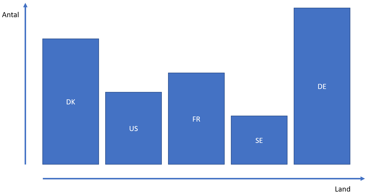
What you are seeing in that picture is a histogram - you are just describing the data distribution with some bars: the higher the bar is, the more records you have for that specific column value. And the same concept and format is used by SQL Server. Let’s have now a look on a more concrete example. In the AdventureWorks2012 database you have the table SalesOrderDetail and within that table you have the column ProductID. That column stores the ID of the product that was part of that specific sale.

In addition there is also an index defined on that column - means that SQL Server has also created a statistics object that describes the data distribution within that column. You can have a look into the statistics object by opening the properties window of it within SQL Server Management Studio, or you can use the command DBCC SHOW_STATISTICS to return the content of the statistics object in a tabular format:

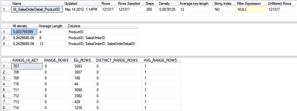
As you can see from the previous screen shot, the command returns you 3 different result sets:

1. General information about the statistics object
2. Density Vector
3. Histogram

Density Vector

Let’s have a look on this mysterious density vector. When you have a look on the Non-Clustered Index IX_SalesOrderDetail_ProductID, the index is only defined on the column ProductID. But in every Non-Clustered Index SQL Server also has to stored the Clustered Key at least as a logical pointer in the leaf level of the index. When you have defined a Non-Unique Non-Clustered Index, the Clustered Key is also part of the navigation structure of the Non-Clustered Index. The Clustered Key on table SalesOrderDetail is a composite one, on the columns SalesOrderID and SalesOrderDetailID.

This means that our Non-Unique Non-Clustered Index consists in reality of the columns ProductID, SalesOrderID, and SalesOrderDetailID. Under the hoods you have a composite index key. This also means now that SQL Server has generated a density vector for the other columns, because only the first column (ProductID) is part of the histogram, that we have already seen in the earlier section. When you look at the output of the DBCC SHOW_STATISTICS command, the density vector is part of the second result set that is returned:

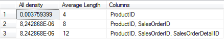
SQL Server stores here the selectivity, the density of the various column combinations.For example, we have an All Density Value for the column ProductID of 0,003759399. You can also calculate (and verify) this value at your own by dividing 1 by the number of distinct values in the column ProductID:

SELECT 1 / CAST(COUNT(DISTINCT ProductID) AS NUMERIC(18, 2))
FROM Sales.SalesOrderDetail
GO

The All Density Value for the column combinations ProductID, SalesOrderID and ProductID, SalesOrderID, SalesOrderDetailID is 8,242867858585359018109580685312e-6. You can again verify this, by dividing 1 by the number of distinct value in the columns ProductID, SalesOrderID, or ProductID, SalesOrderID, SalesOrderDetailID. In our case these values are unique (because they are part of the Clustered Key), so you calculate 1 / 121.317 = 8,242867858585359018109580685312e-6.

Summary

Today you have seen how SQL Server internally structures a statistics object. The most important thing here is the Histogram and the Density Vector, which are used all the time for the cardinality estimation. I hope that you have enjoyed this installment of the SQL Server Performance Tuning series.

Next week we will continue by talking about specific problems with the cardinality estimation in SQL Server, and how to solve them. See you very soon.